OSPFv2 Single-Area

OSPFv2 Single-Area — consolidated study day

This day merges former Days 26, 27 into one CCNA v2.0-aligned segment.

Read straight through; use the practice hub (subnetting / CLI) to drill the verbs Troubleshoot, Diagnose, Configure, and Interpret.

From former Day 26

Source material retained from the previous Day 26 chapter for continuity.

OSPF areas idea

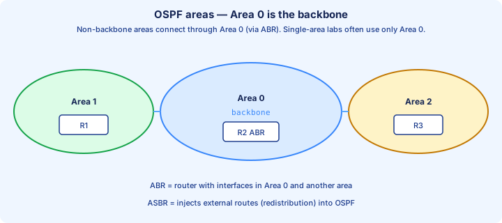
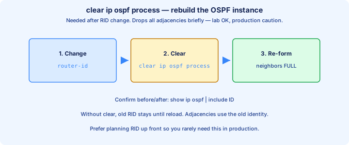
OSPF splits an AS into areas so LSA flooding and SPF stay bounded. Every multi-area design needs Area 0 (the backbone). Non-backbone areas connect through Area 0 via ABRs, not by chaining Area 1 directly to Area 2 as a transit shortcut.

Routers in the same area share the same detailed topology view for that area. Inter-area prefixes arrive as summary LSAs from ABRs. Keeping leaf sites in their own areas shrinks the blast radius when a single link flaps hard.

Single-area labs put every interface in area 0. That is valid and common on CCNA Part 1. Multi-area rules still appear in conceptual questions even when your Packet Tracer topology only configures one area. Still be ready to explain why Area 0 must sit between nonbackbone areas.

Exam trap: two areas can both run OSPF and still black-hole each other if neither touches Area 0 through an ABR.

Router ID

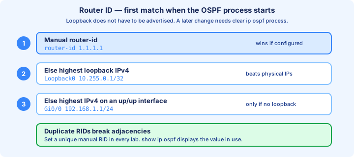
The Router ID (RID) uniquely identifies the OSPF router process. Cisco picks a manual `router-id` first, else the highest up/up loopback IP, else the highest up/up physical IP. Set the RID on purpose in every lab.

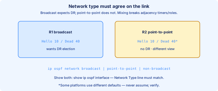
Config: `router ospf 1` then `router-id 1.1.1.1`. Changing RID often needs `clear ip ospf process` (disruptive) before neighbors see the new identity. Duplicate RIDs break adjacency or create LSDB confusion that is hard to spot.

`show ip ospf` prints the active RID. Stable loopbacks make the RID independent of which WAN link is currently up. Document RIDs the same way you document process IDs and area maps.

Exam trap: a higher physical IP does not win if a loopback is up. Loopback beats physical in the automatic election.

Hello / Dead

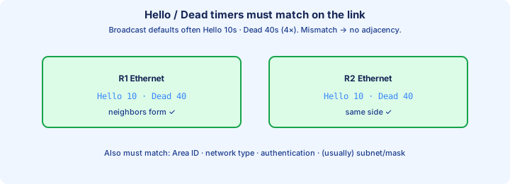
Hello packets discover and maintain neighbors. The Dead interval is how long you wait without hearing a Hello before declaring the neighbor down. Defaults on broadcast and point-to-point Ethernet are often Hello 10 / Dead 40 (Dead = 4 × Hello).

Timers must match on the shared link. A 10/40 router will not form adjacency with a 5/20 peer even if areas match. Set both sides with `ip ospf hello-interval` and `ip ospf dead-interval`, or fix the network type that silently changed the defaults on one end.

`show ip ospf interface` shows Hello and Dead for each OSPF-enabled interface. The neighbor table’s Dead countdown is what you watch when Hellos stop arriving after a shut or ACL change.

Exam trap: mismatched Hello/Dead prevents adjacency even when Area ID and RID look perfect.

Neighbors vs adjacency

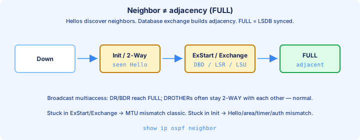
A neighbor is a router whose Hellos you see and accept. A full adjacency means databases are synchronized and you exchange LSAs as adjacency peers (Full state). On multiaccess segments, not every neighbor is Fully adjacent with every other router.

States progress through Down, Init, 2-Way, ExStart, Exchange, Loading, and Full. Stuck in 2-Way on a LAN can be normal for DROthers facing each other. Stuck in ExStart or Exchange often means an MTU mismatch on the link.

`show ip ospf neighbor` shows state per peer. You want FULL/DR, FULL/BDR, or FULL/DROTHER as appropriate for the role. Init-only means Hellos are one-way or parameters still clash.

Exam trap: 2-Way between two DROthers is expected. Panic only when you needed Full and never left 2-Way with the DR.

DR BDR on multiaccess

On broadcast multiaccess (Ethernet), OSPF elects a Designated Router (DR) and Backup DR (BDR) so routers do not full-mesh every adjacency. Others become DROthers and form Full adjacency only with the DR and BDR.

Election uses highest interface priority first (default 1; 0 means ineligible), then highest RID as the tiebreaker. `ip ospf priority` on the interface steers the race. A better latecomer does not instantly preempt an existing DR in classic behavior—boot order matters. Priority 0 is the clean way to keep an access router out of the DR race.

Point-to-point links skip DR election entirely. Hub-and-spoke NBMA designs need careful network types and priorities so the hub becomes DR when the topology requires it.

Exam trap: highest RID wins only when priorities tie. Priority 0 never becomes DR or BDR.

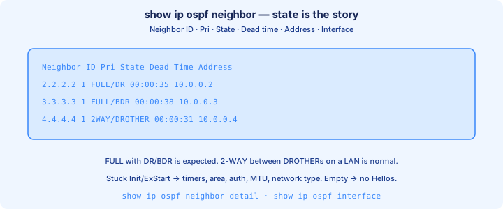
show ip ospf neighbor

`show ip ospf neighbor` lists Neighbor ID (RID), priority, state, Dead timer, peer address, and local interface. It is the first OSPF health command you should run after any adjacency-related config change.

Read the state column against the network type. Full with the DR and BDR on Ethernet is success for a DROther. Missing neighbors means area mismatch, timers, authentication, passive, or a `network` statement that never matched. FULL to the DR is the LAN success criteria for a DROther.

Compare Neighbor ID to `show ip ospf` on the peer so your RID documentation matches reality. The Address column is the peer’s interface IP on that segment, not always the same value as the RID.

Exam trap: Neighbor ID is the RID; the Address column is the link IP. Do not confuse the two on drag-and-drop outputs.

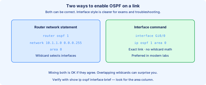
network command vs interface

Legacy style: `router ospf 1` then `network 10.1.1.0 0.0.0.255 area 0`. The wildcard selects local interfaces whose IPs match; those interfaces join that area. Remote subnets are learned from neighbors, not listed in the `network` line.

Interface style: under `interface Gi0/0` use `ip ospf 1 area 0`. It is explicit, hard to over-match, and preferred in modern configs. Both styles can coexist; clarity beats clever wildcards on exam sims.

`show ip ospf interface brief` shows which interfaces are in which area. If an interface is missing, neither the network statement nor the interface command covered it—or the interface is passive or down.

Exam trap: `network` wildcards that are too broad silently enable OSPF on management interfaces you meant to leave quiet.

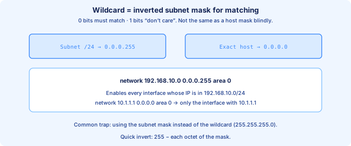
Wildcard masks

An OSPF wildcard is the inverse of a subnet mask for matching: `0.0.0.255` matches a /24 of host bits. `0.0.0.0` matches one host address exactly—useful when you want to pin a single interface IP into an area.

Example: interface 10.1.1.1/24 → `network 10.1.1.0 0.0.0.255 area 0` or `network 10.1.1.1 0.0.0.0 area 0`. The host form cannot accidentally include another interface whose address sits in the same /24 in a messy lab rack.

Do not confuse ACL wildcards’ care/don’t-care logic with wanting to advertise remote networks. Again, you only match local interface addresses into the OSPF process.

Exam trap: writing a subnet mask (`255.255.255.0`) in the `network` statement is wrong; OSPF wants the wildcard (`0.0.0.255`).

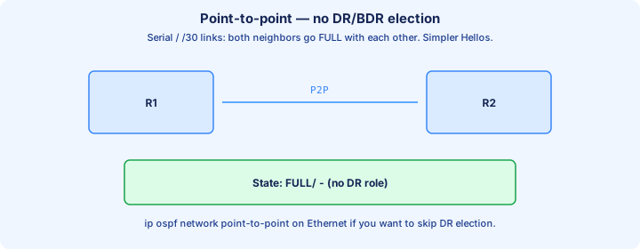
Point-to-point

Point-to-point OSPF network type fits serial links and many Ethernet router-to-router links where only two OSPF speakers exist. There is no DR/BDR election; timers are often Hello 10 / Dead 40 on Ethernet P2P as well, with Fast Hello options on some platforms.

Set with `ip ospf network point-to-point` when default broadcast behavior is wrong for the design—common on Ethernet where you refuse unnecessary DR elections between exactly two routers.

`show ip ospf interface` reports the configured network type. Mismatched types (broadcast versus point-to-point) on the two ends can break adjacency even when areas and RIDs match cleanly.

Exam trap: two routers on Ethernet can stay broadcast and elect a DR needlessly. Point-to-point removes DR from that link.

Cost = bandwidth

OSPF cost defaults from interface bandwidth: cost = reference bandwidth / interface bandwidth (classic reference 100 Mbps). FastEthernet often costs 1; a 10 Mbps link costs 10. Higher cost is worse when SPF adds the path.

Gigabit and faster links all cost 1 under a 100 Mbps reference, so OSPF cannot prefer 10G over 1G until you raise `auto-cost reference-bandwidth` on every router consistently or set `ip ospf cost` manually on the interfaces. Raise reference bandwidth everywhere or costs stay tied at one on fast links.

`show ip ospf interface` displays the cost in use. Path cost is the sum of outbound interface costs toward the destination. Lowest total wins among intra-area candidates for that prefix.

Exam trap: changing bandwidth on an interface changes OSPF cost. Changing delay does not—that is an EIGRP lever.

Router types ABR ASBR

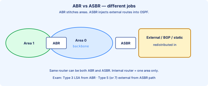
An internal router has all OSPF interfaces in one area. An ABR (Area Border Router) connects Area 0 to at least one other area and originates inter-area summaries. An ASBR injects external routes into OSPF through redistribution.

A single box can be both ABR and ASBR. `show ip ospf border-routers` and the LSDB reveal those roles in verification. External route types (E1/E2) point back toward ASBRs in later OSPF detail.

Design ABRs carefully: they are the only legal door between a non-backbone area and the rest of the OSPF domain via Area 0. Skipping Area 0 breaks inter-area reachability even if both areas look locally healthy. Label ABRs on your diagram before you troubleshoot missing inter-area routes.

Exam trap: a router with interfaces only in Area 1 and Area 2, and none in Area 0, is not a valid ABR path between those areas.

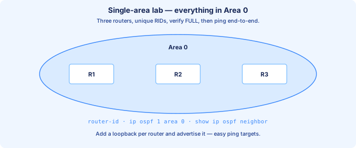
Single area lab

Lab three routers with all interfaces in area 0. Set unique RIDs, enable OSPF with interface `ip ospf 1 area 0` or tight network statements, and ensure each link shares a subnet. Skip DR drama on P2P; on a switched LAN segment, watch which router wins DR.

Pass criteria: `show ip ospf neighbor` shows Full, `show ip route ospf` lists remote LANs with O codes, and pings succeed host to host across the lab. Save configs only after that set is clean.

Break it on purpose: mismatch an area ID on one link, fix it, then mismatch Hello timers. Muscle memory for Day 26 is adjacency first, installed routes second, ping third.

If neighbors never form, do not chase cost values. Fix area, timers, masks, and `network`/interface enablement before SPF tuning.

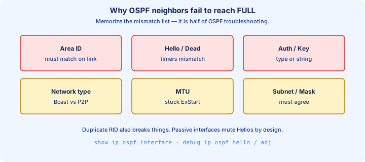
Common adjacency blocks

Frequent blockers: mismatched area ID, Hello/Dead timers, authentication, stub flags, MTU, network type, duplicate RID, passive interface, ACL dropping 224.0.0.5/6, and subnet mask mismatch on the shared link.

Layer 1/2 down is still the boring winner. Confirm `show ip ospf interface` lists the interface as up and non-passive before deep theory. Unique RIDs and matching timers fix a surprising share of student labs. Duplicate RID and mask mismatch belong on every adjacency checklist.

MTU mismatch often sticks peers in ExStart or Exchange. `ip ospf mtu-ignore` is a lab bandage; matching MTU on both ends is the real fix you should take into production habits.

Exam trap: same subnet is required. 10.1.1.1/24 peering 10.1.1.2/30 is a classic silent failure.

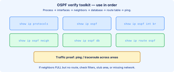
Verification set

Order the checks: `show ip ospf` for RID and process, `show ip protocols` for networks and passives, `show ip ospf interface brief` for area membership and cost, `show ip ospf neighbor` for state, then `show ip route ospf` for installed paths.

Add `show ip ospf database` when neighbors are Full but a prefix is missing—confirm the LSA exists before you blame the RIB. Ping and traceroute validate forwarding only after the control plane looks right.

Capture before/after output when you clear OSPF or shut a link. Convergence time and alternate costs should match what the drawn topology predicts for that failure.

Exam trap: routes without Full adjacency to the needed DR or point-to-point peer are incomplete. Neighbor table before RIB.

From former Day 27

Source material retained from the previous Day 27 chapter for continuity.

LSA types overview

An LSA is a Link-State Advertisement. OSPF routers flood LSAs inside an area so every router builds the same LSDB (link-state database), then runs SPF. The type number tells you what the LSA describes and how far it is allowed to travel.

CCNA needs Type 1 (Router), Type 2 (Network), Type 3 (Summary from an ABR), and awareness of Type 4 (ASBR summary) and Type 5 (External from an ASBR). Types 1 and 2 stay inside one area. Type 3 crosses ABRs. Type 5 floods the OSPF domain except into stub-style areas.

Do not memorize type numbers in isolation. Ask: who originates it, what prefix or topology it describes, and whether an ABR or ASBR rewrites it when it crosses an area border. That map is what `show ip ospf database` will show you later today.

Exam trap: Type 3 is not “external.” External means redistributed into OSPF as Type 5 (or Type 7 in NSSA). Type 3 is an inter-area summary from an ABR.

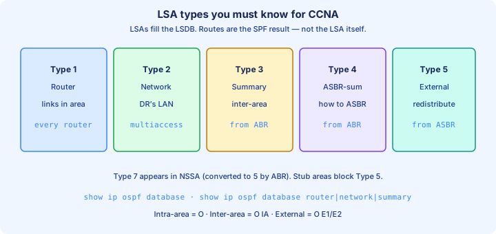
Type 1 2 3

Type 1 Router LSA: every OSPF router originates one per area it belongs to. It lists that router’s links in the area—stub nets, transit nets, and point-to-point neighbors—with costs. Link-state ID is usually the originating Router ID.

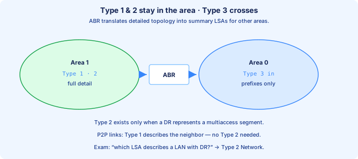
Type 2 Network LSA: the DR on a multi-access segment originates it. It lists the routers attached to that LAN (the DR and its adjacent neighbors). Point-to-point links do not need a Type 2; there is no DR election there.

Type 3 Summary LSA: an ABR advertises a prefix learned in one area into another. Area 1’s prefix appears in Area 0 as a Type 3, not as a full copy of every Type 1/2 from Area 1. That is how multi-area OSPF stays scalable.

Exam trap: a stub router with only one interface in an area still originates a Type 1. Missing Type 2 on Ethernet usually means no DR, wrong network type, or the adjacency never reached Full.

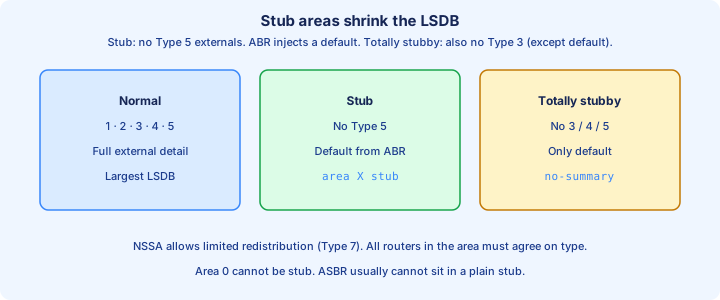
Area types stub intro

A stub area blocks Type 5 external LSAs. Internal routers in the stub do not carry a full external table. The ABR injects a default route (typically as a Type 3 default) so stub routers still reach outside destinations via the ABR.

Configure consistently: `area 1 stub` under the OSPF process on every router in that area, including the ABR. A stub flag mismatch means neighbors will not form. Totally stubby (`area 1 stub no-summary`) also blocks most Type 3s and leaves mainly the default—know the idea; deep NSSA detail is later.

Use stubs for leaf areas with no ASBR of their own. If the area must redistribute or host an ASBR, it cannot be a plain stub. Area 0 is never stub.

Exam trap: stub stops Type 5s; it does not by itself remove all Type 3 inter-area routes. That is the totally stubby option.

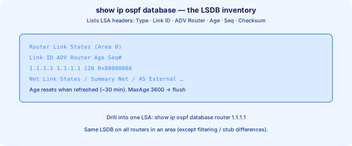
show ip ospf database

`show ip ospf database` is the LSDB inventory. Sections group Router Link States (Type 1), Net Link States (Type 2), Summary Net Link States (Type 3), and external types when present. Columns show Link ID, ADV Router, Age, Seq#, and Checksum.

Confirm the ADV Router matches the RID you expect. On an internal Area 1 router you should see local Type 1/2 for Area 1 and Type 3s from the ABR for remote prefixes. On the ABR, expect Type 1s for each area it belongs to and Type 3s it originates into the other area.

Drill with filters: `show ip ospf database router`, `show ip ospf database network`, `show ip ospf database summary`. Age climbing toward 3600 without refresh means a router stopped updating that LSA. Seq# jumps after a topology change.

Exam trap: the RIB can look empty while the LSDB is full, or the reverse after filtering. Always pair `show ip ospf database` with `show ip route ospf`.

Inter-area routes

An inter-area route is a prefix learned from another OSPF area via a Type 3. In `show ip route` it codes as O IA. The next hop is toward the ABR that advertised the summary into your area.

Intra-area paths use the full Type 1/2 topology and SPF inside the area. Inter-area paths treat the ABR as the exit, then use the metric advertised in the Type 3 plus the cost to that ABR. You do not re-run SPF across the remote area’s full graph.

ABRs connect areas to backbone Area 0. Non-backbone areas should touch Area 0 (directly or via a virtual link—Day 28). Without a path through Area 0, inter-area reachability breaks even if each island looks Full locally.

Exam trap: O IA means inter-area OSPF, not “inactive” or “incomplete adjacency.” Full neighbors can still lack O IA if the ABR never originated the Type 3.

Intra-area preference

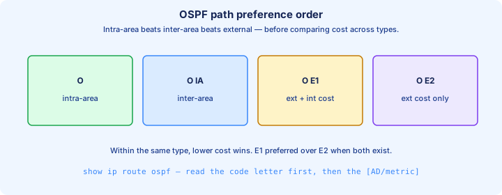
OSPF path preference for the same destination: intra-area (O) beats inter-area (O IA), which beats external E1, which beats external E2 (with E2’s tie-breaks on forward metric). Cost alone does not override that order.

If Router A can reach 10.1.1.0/24 as O via a long intra-area path and as O IA via a short ABR path, it still prefers O. Design areas so the preferred path is the one you intend, or you will chase “wrong” next hops that are protocol-correct.

Prove it in the lab: advertise the same prefix both ways, then read `show ip route 10.1.1.0`. The code letter and the “from” / via lines tell you which rule won. Do not assume lowest cost always wins across path types.

Exam trap: a lower-cost O IA does not beat a higher-cost O for the same prefix. Path type first, then cost within that type.

Passive interface

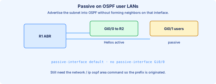
`passive-interface GigabitEthernet0/2` under the OSPF process stops Hellos on that interface. The connected subnet is still advertised into OSPF. No adjacency forms on that link. Use it on LAN interfaces facing PCs and on any edge where you must inject the prefix without peering.

Best habit: `passive-interface default` then `no passive-interface` on the few links that should neighbor. That prevents accidental Hellos on every new SVI. Confirm with `show ip ospf interface brief`—passive interfaces show no neighbor expectation.

Passive is not the same as removing `network` or `ip ospf` from the interface. Remove the interface from OSPF and the subnet disappears from LSAs. Passive keeps the prefix, drops the Hello.

Exam trap: passive on a link between two routers means they never become neighbors, even though each may still advertise its own side of the subnet if that subnet is in OSPF elsewhere.

Default route injection

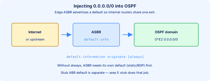
OSPF does not redistribute a default just because you typed `ip route 0.0.0.0 0.0.0.0 …`. Inject it with `default-information originate` under the OSPF process on the ASBR (or edge ABR role in a lab). Neighbors then install an O*E2 (or similar) default toward that injector.

By default, originate requires a default already in the local RIB. Add `always` to advertise 0.0.0.0/0 even when the injector has no default of its own—useful in labs, dangerous if the uplink is actually down.

Stub areas get a default from the ABR as part of stub behavior; that is separate from `default-information originate` for externals. Know which mechanism is in play before you chase missing defaults.

Exam trap: `default-information originate` without a candidate default (and without `always`) injects nothing. Check the ASBR’s RIB first.

MTU mismatch

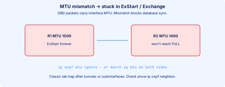
OSPF includes interface MTU in DBD packets during ExStart/Exchange. If MTUs differ, neighbors often stick in ExStart or Exchange and never reach Full. Ping may still work; the control plane is what fails.

Symptoms: `show ip ospf neighbor` stuck short of Full, log messages about MTU mismatch, or repeated DBD retransmits. Fix by matching `ip mtu` / interface MTU on both sides, or (lab only) `ip ospf mtu-ignore` on the interface—prefer fixing MTU for production habits.

Common lab cause: one side has a subinterface or tunnel MTU shaved, the other is default 1500. Ethernet to Ethernet should match unless you intentionally changed it.

Exam trap: MTU mismatch is the classic ExStart/Exchange stuck case. Timer mismatch usually prevents neighborship earlier; do not mix the two stories.

Timers mismatch

Hello and Dead timers must match on the shared segment. Defaults depend on network type: often Hello 10 / Dead 40 on broadcast and point-to-point, Hello 30 / Dead 120 on non-broadcast. Change with `ip ospf hello-interval` and `ip ospf dead-interval`.

If timers disagree, Hellos are ignored and the neighbor never appears, or flaps. `show ip ospf interface` prints the timers in use. Match both ends; do not assume “faster Hellos always help” without changing Dead in proportion.

Network-type changes often change timers for you. Setting `ip ospf network point-to-point` on one side and leaving broadcast on the other can create a timer-looking failure that is really a type mismatch.

Exam trap: Dead must be greater than Hello. Matching Hello but leaving Dead mismatched still breaks the adjacency requirements on many platforms.

Network type mismatch

OSPF network type controls DR election, multicast behavior, and default timers. Common types: broadcast, point-to-point, non-broadcast, point-to-multipoint. Ethernet defaults to broadcast; serial often point-to-point.

If one side is broadcast (expects DR/BDR) and the other is point-to-point (no DR), adjacency may fail or act oddly. `show ip ospf interface` shows Network Type and whether a DR exists. Set both ends the same with `ip ospf network …`.

Point-to-point on Ethernet between two routers is a common lab choice: no DR election, faster bring-up, /30 or /31 still works. Just configure both sides.

Exam trap: 2-Way between DROTHERs on a healthy broadcast LAN is normal. 2-Way when you expected Full to the DR is not a network-type success story—check priority, timers, and type match.

Clear ip ospf process

`clear ip ospf process` restarts the OSPF process: neighbors drop, LSDBs rebuild, SPF runs again. It is disruptive. Use it in labs after RID changes, stubborn DR elections, or when you need a clean adjacency cycle—not as a daily “fix.”

IOS prompts for confirmation. On multi-area routers every area’s adjacencies bounce. Prefer clearing a single neighbor or bouncing one interface when the problem is local: `clear ip ospf neighbor` variants or `shutdown` / `no shutdown` on the link.

After a clear, watch `show ip ospf neighbor` return to Full and re-check `show ip route ospf`. If the bad state returns immediately, the clear proved the config is still wrong—fix the cause, do not clear again on a loop.

Exam trap: clearing OSPF does not fix MTU, timer, area, or authentication mismatches. It only forces renegotiation under the same broken config.

Lab multi-area

Build Area 0 between R1–R2 and Area 1 beyond an ABR (R2). Put a loopback or LAN in Area 1 and another in Area 0. Enable OSPF with correct `network … area` statements or interface `ip ospf` commands so each interface lands in one area only.

Pass criteria: neighbors Full in each area, Area 1 router shows O IA for Area 0 prefixes, Area 0 router shows O IA for Area 1 prefixes, and `show ip ospf database` shows Type 3s originated by the ABR. Ping end-to-end.

Optional stretch: make Area 1 stub on all Area 1 routers and the ABR, confirm Type 5s (if any) vanish from the stub LSDB, and confirm a default appears. Capture before/after `show ip route ospf`.

If O IA is missing, verify the ABR is in both areas, Area 0 is present, and the ABR’s Type 3 section lists the prefix before you touch timers.

Exam traps

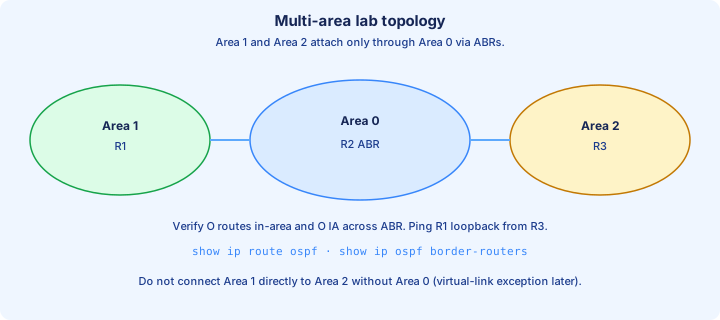
Stack these traps: Type 3 ≠ external; O preferred over O IA; stub blocks Type 5 not (by itself) all Type 3; passive advertises without Hellos; MTU → ExStart/Exchange; timers/network type → no stable neighbor; clear process is not a config fix.

DR sticky behavior: raising priority does not instantly steal DR. Old DR stays until it leaves. Labs may need a bounce or `clear ip ospf process` after priority surgery—know that story for Day 28 as well.

Verification order under pressure: `show ip ospf neighbor` → `show ip ospf interface` → `show ip ospf database` → `show ip route ospf`. Match area ID, timers, MTU, and network type before you redesign the area plan.

Exam trap: two routers in Area 1 with no ABR to Area 0 can be Full to each other and still have no inter-area routes to the rest of the network.